
- Projection structure of the Green-Naghdi model
The numerical resolution of the dispersive models are still nowadays an scientific chalenge. Some of them and in particular the Green- Naghdi model, present a structure of projection. More precisely, following the example of the incompressible models, the time-discrete Green-Naghdi model can be define as the projection of the solution of the shallow water model on a set of admissible functions [3]. This observation allows the construction of schemes that preserve important properties of the model, i.e. the entropy stability and the preservation of the steady state, see next figure. The figure shows the steady state of the Green-Naghdi model defined as orbites around the state at rest (brown line) and wrapped by the steady soliton solution (dashed red line). The projection structure is also way to define well-posed boundary conditions. Last but not least, it allows to reduce the numerical cost by applying the projection only where and when the Green-Naghdi model differs significantly from the shallow water model, via an a priori estimator.
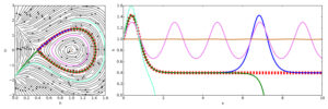
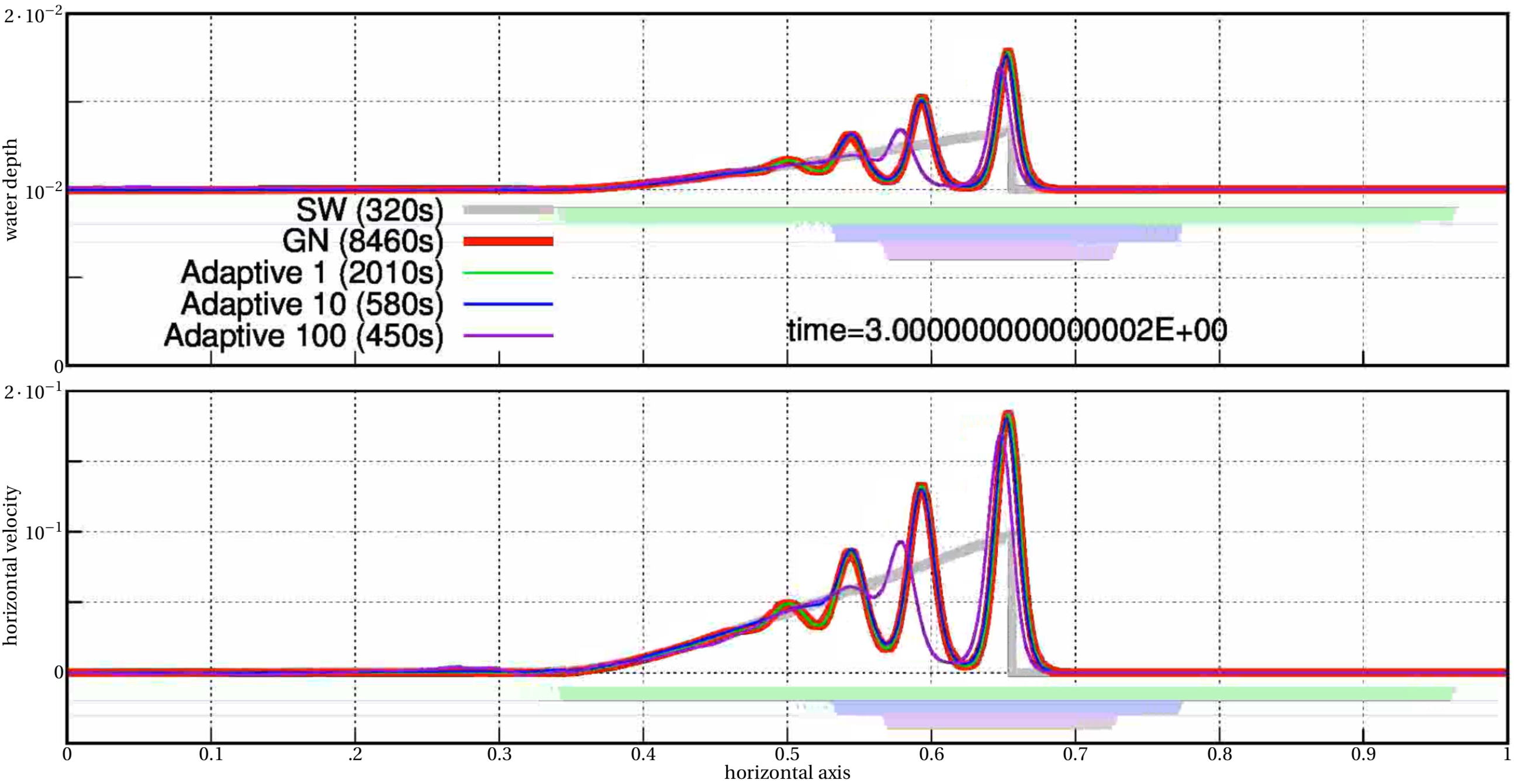
This strategy is illustrated in the second figure. This strategy required a numerical parameter, corresponding to the admissible error and the more this error is small, closer to the Green-Naghdi model the solution will be.
The figure presents the simulation of the propagation of waves with the shallow water model (SW), the Green-Naghdi model (GN) and an adaptive strategy between the two models. The colored areas below the curves represent the domain where the projection is applied.In the considering simulation, it was possible to get a result almost exactly fitting with the Green-Naghdi model with a CPU time fourth time smaller. - The “splitting” method
We work on hybrid strategies for the solution of the Green-Naghdi system of equations, for the simulation of the fully nonlinear weakly dispersive free surface waves, on unstructured meshes. We consider a two step solution procedure composed of a first step where the non-hyrostatic source term is recovered by inverting an elliptic coercive operator associated to the dispersive effects; a second step which involves the solution of the hyperbolic shallow water system with the source term, computed in the previous phase, which accounts for the non-hydrostatic effects. See [1] and [2] for more info. Any appropriate numerical method can be used to discretise the two stages.
References
- A. Filippini, M. Kazolea and M. Ricchiuto. A flexible genuinely nonlinear approach for wave propagation, breaking and runup. J.Comput.Phys., 310:381–417, 2016. (PDF)
- M. Kazolea, A.G. Filippini, and M. Ricchiuto. A low dispersion finite volume/element method for nonlinear wave propagation, breaking and runup on unstructured meshes, submitted to Ocean Modelling, https://hal.inria.fr/hal-03402701
- E. D. Fernandez-Nieto, M. Parisot, Y. Penel, J. Sainte-Marie. A hierarchy of dispersive layer-averaged approximations of Euler equations for free surface flows. Communications in Mathematical Sciences, International Press, 2018, 16 (5), pp.1169-1202. https://dx.doi.org/10.4310/CMS.2018.v16.n5.a1