
- A Layerwise dispersive model
The master model of free surface flows is the so-called Water Waves model. Unfortunately, this model is too costly to solve numerically at the scale of the geophysical applications, i.e. harbor or costal area. The shallow water model is a good approximation of the incompressible Navier-Stokes system with free surface and it is widely used for its mathematical structure and its computational efficiency. However, this model suffer of two drawbacks: it does not take into account the hydrodynamic pressure and it does not take into account the vertical variation of the horizontal velocity. Several models propose an advanced version of the shallow water model to take into account the hydrodynamic pressure, and the most famous is the Green Naghdi model. In parallel, some discretization techniques allow the vertical description of the horizontal velocity, such as the layerwise shallow water model. Putting this two techniques together, we propose a hierarchy of model, so called the layerwise Green-Naghdi model [3]. To illustrate the efficiency of the layerwise Green-Naghdi model, we compute its dispersion relation for some number of layers, see figure on the left. The plot shows the dispersion relations of the hierarchy of models. (Csw ) is the dispersion relation of the shallow water model. (C-NHL ) is the dispersion relation of the layerwise Green-Naghdi model with L-layers.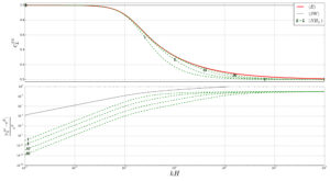 A good dispersion relation is essential to reproduce the propagation of waves. We show that the dispersion relation of the layerwise Green-Naghdi model converge to the dispersion relation of the Water Waves model when the number of layers goes to infinity. Next we present the numerical results obtained with the different models for a wave passing over a dike. The first picture (T0) shows the initial condition. The second picture (T1) shows the response of the models to the bottom variation: the dispersive models are quite similar and regular while the solution of the shallow water model is discontinuous. The third picture (T2) shows the solutions when the shallow water model passes over the dike: the solution of the shallow water is regular. The fourth picture (T3) shows the solutions when the dispersive model pass over the dike: the solution of the dispersive models is very stiff. The fifth picture (T4) shows the solutions after the dike: the solution of the classical Green-Naghdi model (N H 1 ) is significantly faster than the models with more layers.
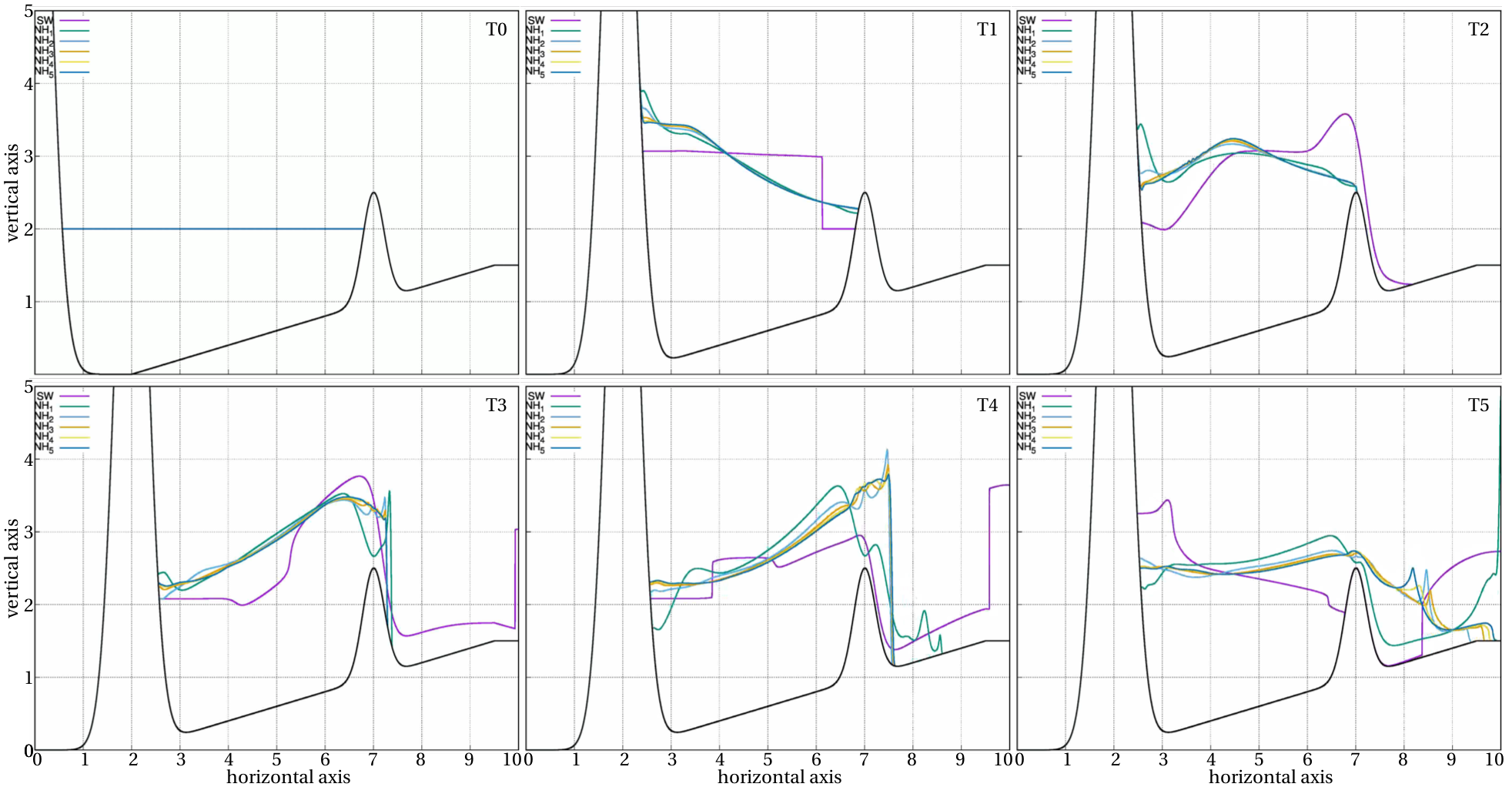
 SW ) curve is the numerical result with the shallow water model. (NHL) curves are the numerical results with the layerwise Green-Naghdi model with L-layers. We can explain this observation by the presence of vortices trapping part of the wave energy without contributing to its propagation for the model with several layers.
- Enhanced Highly non-linear dispersive models
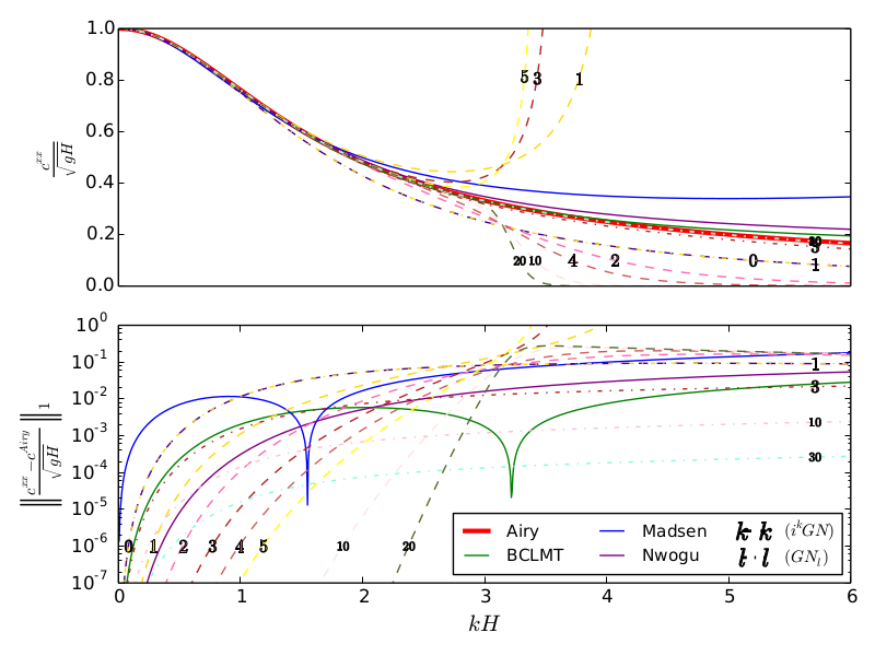
We currently work to improve the dispersion relation of highly non-linear weakly dispersive models. By improving we mean that we want to approximate the Airy dispersion relation.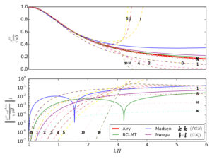 Some preliminary results can be shown in the next picture. More precisely the picture shows the celerity of different weakly dispersive models. Red Line indicates the dimensionless celerity of the Euler equations, blue line the one of the Madsen and Sorensen equation, purple line refers to Nwogu’s equation and all the dashed lines to improved Green-Naghdi equations. This is a work in progress.
- Boundary conditions for the Green-Naghdi weakly dispersive fully nonlinear model
In order to preserve the projection structure of the equations [1] on a bounded domain, it is possible to show that a class of boundary conditions have to satisfy a Dirichlet boundary condition either on the velocity, either on the hydrodynamic pressure. This strategy follows a classical strategy used in the case of the incompressible flows (Stokes or Navier-Stokes), with a particular admissible function set and scalar product. It is also possible to deal with a dry front as a particular boundary condition for the projection step. Next video shows a solitary wave passing through the boundaries of the domain without any reflection. For more information the reader is referred to [2].
References
- M. Parisot. Entropy-satisfying scheme for a hierarchy of dispersive reduced models of free surface flow. Int J Numer Meth Fluids. 2019; 91: 509– 531. https://doi.org/10.1002/fld.476S. Noelle, M.
- S. Noelle, M. Parisot, T. Tscherpel. A class of boundary conditions for time-discrete Green–Naghdi equations with bathymetry. SIAM Journal on Numerical Analysis. https://arxiv.org/pdf/2106.05048.pdf
- E. D. Fernandez-Nieto, M. Parisot, Y. Penel, J. Sainte-Marie. A hierarchy of dispersive layer-averaged approximations of Euler equations for free surface flows. Communications in Mathematical Sciences, International Press, 2018, 16 (5), pp.1169-1202. https://dx.doi.org/10.4310/CMS.2018.v16.n5.a1