Ice release is of concern to aircraft manufacturers due to the potential damage that the ice debris can cause on aircraft components. Impact of large ice debris on downstream aerodynamic surfaces and ingestion by aft mounted engines must be considered during the aircraft certification process. This raises the need for accurate ice trajectory simulation tools to support pre-design, design and certification phases while improving cost efficiency.
There are generally two types of model used to track shed ice pieces, which are distinguished by their level of fidelity. The first type of model (low-fidelity) makes the assumption that ice pieces do not significantly affect the flow field, and the second type of model (high-fidelity) intends to take into account ice pieces interacting with the flow. High-fidelity models involve fully coupled time-accurate aerodynamic and flight mechanics simulations and thus require the use of emerging simulation tools, such as approaches based on immersed boundary methods or chimera grids. Cardamom team proposes to model ice shedding trajectories by an innovative paradigm that is based on penalization and level-sets.
Penalization is an efficient alternative to explicitly impose boundary conditions so that the body-fitted meshes can be avoided, making multifluid/multiphysics flows easy to set up and simulate. Level sets describe the geometry in a nonparametric way so that geometrical and topological changes due to physics and in particular shed ice pieces are straight forward to follow. The capabilities of the proposed model are demonstrated on ice trajectories calculations in the flow around an airfoil, figure 1.
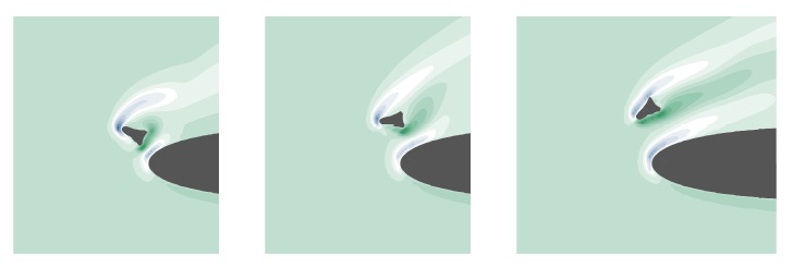
Figure1. Vorticity contours and ice block trajectory around a Naca 0012 airfoil
The drawbacks of embedded techniques are the treatment of wall boundaries. To overcome this difficulty, we have an extension of penalisation for compressible flows to unstructured adaptive grids. This allows to use mesh adaptation to insure an accurate treatment of the wall boundary condition. The idea is then to combine the strength of mesh adaptation to the simplicity of embedded grids techniques. The concept has been used both in 2D and in 3D, and both for steady and time dependent flows. Figure 2 for example shows the case of a laminar supersonic computation around a 2D wedge. A similar computation has been performed in 3D, involving the flow around an extruded wedge of finite length. Figure 3 shows the type of mesh obtained in this case, and the benefit in terms of resolution of the flow.
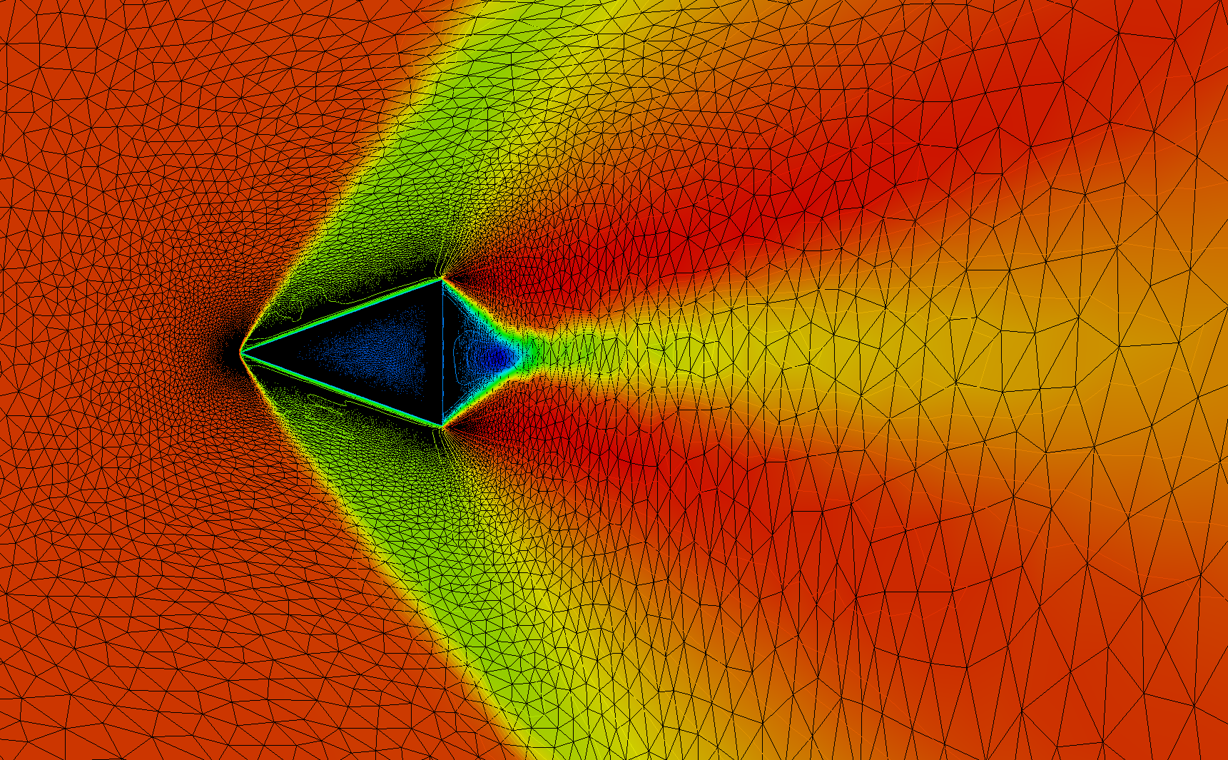
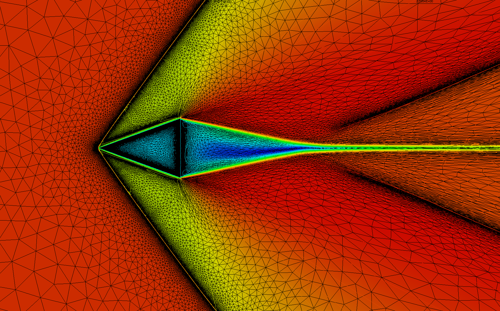
Figure 2. 2D supersonic triangle : u velocity on initial and adapted mesh
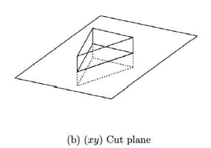
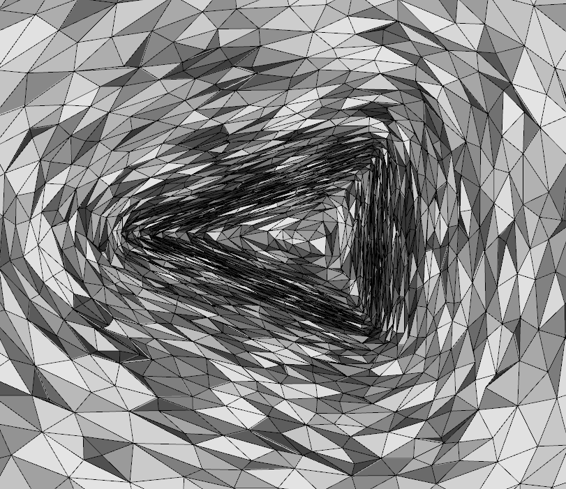

Figure 3. 3D extruded wedge. adapted mesh in the transversal section
We consider two extensions. The first is to time dependent flows, which been performed using adaptation techniques based on mesh deformation (r-adaptation). In this case, and initial (possibly adapted) mesh is deformed using an elliptic PDE whose coefficients (and/or right-hand-side) depend on the flow being computed. In this case, adaptation w.r.t. the zero level set, and w.r.t. some flow smoothness indicator is performed. The typical result is shown in the videos below showing the vorticity generated by a flapping Naca airfoil, and the mesh obtained with the adaptation approach proposed. The validation of the forces computed on the body is also reported.

Flapping NACA0012 airfoil: drag force
The second extension considers computations with high order elements and adaptive meshes have been performed using AEROSOL and MMG. A first example involves the separated 3D laminar flow around a sphere at Reynolds number 300. Immersed P2 computations are performed using mesh adaptation w.r.t. both the zero level set (representing the exact position of the sphere), and the flow (Mach number). Below a view of the adapted mesh, of the Mach number and of the streamlines. The last two allow to compare the immersed computation to a P2 conformal one. The two are almost indistinguishable.

The corresponding separation angles, separation length, and position of the center of the recirculation bubble on the symmetry plane are reported in the table below are compare well to the reference by Johnson and Patel J.Fluid Mech. 378. 1999.

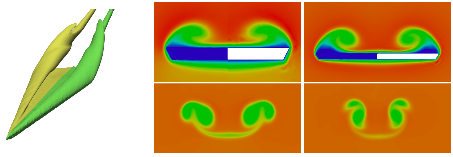
Another example is the following flow around a delta wing, featuring a highly separated laminar flow with strong vortical structures appearing behind the body. Mesh adaptation is again performed with respect to both the zero level set position and to the Mach Number. A visualization of the neat capturing of the vortical structures obtained with a third order P2 simulation is provided below, showing the adapted mesh superimposed to the Mach iso-surfaces.

A comparison between the P2 immersed computation to a P2 conformal one are reported hereafter. The left 3D picture shows the roll-up of primary and secondary vortices in 3D (left half conformal, right half immersed computation). The right pictures compare the evolution of the vortical structures in space via the Mach number distribution at x = 0.5C, x = C, x = 1.5C and x = 2C. The adaptive immersed and conformal results are nearly identical.