


by Chris Reinke and Xavier Alameda-Pineda
Transactions on Machine Learning Research
Abstract. Transfer in Reinforcement Learning aims to improve learning performance on target tasks using knowledge from experienced source tasks. Successor features (SF) are a prominent transfer mechanism in domains where the reward function changes between tasks. They reevaluate the expected return of previously learned policies in a new target task and to transfer their knowledge. A limiting factor of the SF framework is its assumption that rewards linearly decompose into successor features and a reward weight vector. We propose a novel SF mechanism, ξ-learning, based on learning the cumulative discounted probability of successor features. Crucially, ξ-learning allows to reevaluate the expected return of policies for general reward functions. We introduce two ξ-learning variations, prove its convergence, and provide a guarantee on its transfer performance. Experimental evaluations based on ξ-learning with function approximation demonstrate the prominent advantage of ξ-learning over available mechanisms not only for general reward functions but also in the case of linearly decomposable reward functions.
Transfer Learning and Successor Features (SF)
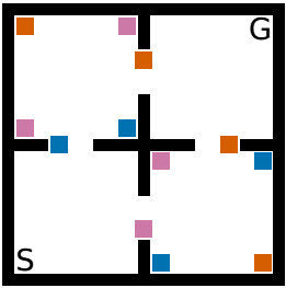 In Reinforcement Learning an agent often needs many interactions with its environment to learn a good behavior. Transfer Learning tries to reduce the required interactions by using knowledge from former learned tasks (source tasks) for the current task (target task). SF is a technique that allows such transfer in tasks where the environment dynamics are the same, but where the reward function changes between tasks. For example, in the object collection task (shown right) introduced by Barretto et al. (2017), the goal of the agent is to collect a number of objects before reaching a goal area (G). The position of the objects and the layout of the environment are fixed, but how much reward the agent gains for an object of a specific type (pink, orange, blue) changes between tasks. SF allows reevaluating how a previously learned policy, for example, one that learned to collect pink and orange objects in a task where these give a high reward, would perform in a task where only pink objects give a high reward. This knowledge is then used to select the best action from all previously learned policies by reevaluating them in the new target task.
![]()
SF was introduced by Barretto et al. (2017). It works by decomposing the rewards and dynamics in a task. The reward function is described by a linear composition of rewards r into features φ and a reward weight vector w:For the object collection task, the features are a binary vector with 4 elements. The first 3 elements describe if an object of a specific type is collected. The last element defines if the goal area is reached. For example, the feature vector for collecting a pink object is φ = [1,0,0,0], a blue object is φ = [0,0,1,0], and reaching the goal state is φ = [0,0,0,1]. The weight vector w defines the rewards that are given for the different situations, for example, w = [0.5, 0.0, -0.25, 1.0] gives a reward of 0.5 for collecting a pink object, 0.0 for an orange object, -0.25 for a blue object, and 1.0 for reaching the goal area.
This linear decomposition of rewards into features and reward weights allows decomposing also the Q-function. The Q-function measures the future expected reward sum if the agent follows a certain behavior. It gets decomposed in a SF function ψ, and the reward weight vector w:
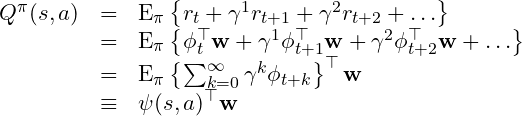 The SF function ψ is a vector function and represents the expected future cumulative successor features that the agent would encounter given its behavior, i.e. the policy the maximizes the current task.
For each new task i, which is defined by a different weight vectors wi, the agent learns a SF function ψi that optimizes task i. Standard Reinforcement Learning Temporal Difference methods such as Q-Learning can be used to learn it. Having learned the optimal SF functions for a set of tasks, the agent can reevaluate their outcome, i.e. the Q-Value, for a new target task j with weight vector wj. It selects the best action a in a state s according to the General Policy Improvement (GPI) theorem:
![]()
ξ-Learning
A problem with classical SF is that it is based on the assumption that the rewards are a linear combination of features and reward weights. Our goal with ξ-learning is to overcome this restriction, by allowing the usage of SF for general reward functions: ![]() We achieve this by learning the expected future cumulative discounted probability over possible features, which we call ξ(Xi)-function. The ξ-function is a discounted sum over the probabilities to see a specific feature at a specific time point t+k:
We achieve this by learning the expected future cumulative discounted probability over possible features, which we call ξ(Xi)-function. The ξ-function is a discounted sum over the probabilities to see a specific feature at a specific time point t+k: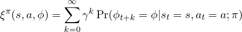 The ξ-function allows to reconstruct the Q-values and therefore to reevaluate previously learned policies for any new general reward function R:
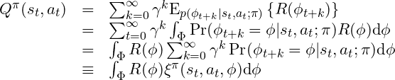
Our paper introduces the theoretical background to ξ-learning, different versions of how to implement it, a proof of its convergence to the optimal policy, and a theoretical guarantee of its transfer performance.
Experiments and Results
We evaluated ξ-learning in 2 environments: 1) In a modified version of the object collection task introduced by Barreto et al. (2017) which has discrete (here binary) features. 2) In a racer environment with continuous features.
1) Object Collection Environment
The environment consists of 4 rooms (a). The agent starts an episode in position S and has to learn to reach the goal position G. During an episode, the agent can collect objects to gain further rewards. Each object has 2 properties: 1) color: orange or blue, and 2) form: box or triangle. The features are binary vectors. The first 2 dimensions encode if an orange or a blue object was picked up. The 2 following dimensions encode the form. The last dimension encodes if the agent reached goal G. For example, φ = [1, 0, 1, 0, 0] encodes that the agent picked up an orange box.
Each agent learns sequentially 300 tasks which differ in their reward for collecting objects. We compared agents in two settings: either in tasks with linear or general reward functions. For each linear task, the rewards are defined by a linear combination of features and a weight vector w. The weights for the first 4 dimensions define the rewards for collecting an object with specific properties. They are randomly sampled from a uniform distribution: wi;k ∼ U(−1; 1). The final weight defines the reward for reaching the goal position which is wi;5 = 1 for each task. The general reward functions are sampled by assigning a different reward to each possible combination of object properties φj using uniform sampling: Ri(φj) ∼ U(−1; 1), such that picking up an orange box might result in a reward of Ri(φ = [1; 0; 1; 0; 0]) = 0.23.
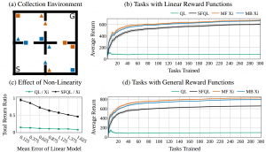
We compared two versions of ξ-learning (MF Xi and MB Xi) to standard Q-learning (QL) that has no transfer and the classical SF procedure (SFQL). In the case of general reward functions, the SFQL receives a weight vector wi for each task that was fitted to best describe the reward function using a linear decomposition. Our results show that ξ-learning has already a minor advantage over SFQL in tasks with linear reward functions (b) and a larger advantage in tasks with general reward functions (d).
We further evaluated the effect of non-linearity in the reward functions on the performance of ξ-learning vs SFQL in (c). The results show the ratio of the total collected reward sum between the SFQL and MF Xi (black line). Each point shows the result for learning over 300 tasks with reward functions that are more and more difficult to approximate with a linear decomposition (as used by SFQL). SFQL can reach a similar performance in tasks that can be relatively well approximated (mean linear reward model error of 0.125), but SFQL has only less than 50% of MF Xi’s performance in tasks with a high non-linearity (mean linear reward model error of 1.625).
2) Racer Environment
We further evaluated the agents in an environment with continuous features. The agent is randomly placed in the environment and has to drive around. Similar to a car, the agent has an orientation and momentum, so that it can only drive straight, or in a right or left curve. The agent reappears on the opposite side if it exits one side. The distances to 3 markers (orange, blue, green) are provided as features. Rewards depend on these distances where each marker has 1 or 2 preferred distances defined by Gaussian functions. For each of the 65 tasks, the number of Gaussian’s and their properties (µ, σ) are randomly sampled for each feature dimension. (a) shows an example of a reward function with dark areas depicting higher rewards. The agent has to learn to drive around in such a way as to maximize its trajectory over positions with high rewards.
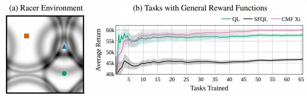
ξ-learning (CMF Xi) reached the highest performance of all agents (b). SFQL reaches only a low performance below QL, because it is not able to sufficiently approximate the general reward functions with its assumption on linearly decomposable reward functions.
Conclusion
In summary, the contribution of our paper is three-fold:
- We introduce a new RL algorithm, ξ-learning, based on a cumulative discounted probability of successor features, and several implementation variants.
- We provide theoretical proofs of the convergence of ξ-learning to the optimal policy and for a guarantee of its transfer learning performance under the GPI procedure.
- We experimentally compare ξ-learning in tasks with linear and general reward functions, and for tasks with discrete and continuous features to standard Q-learning and the classical SF framework, demonstrating the interest and advantage of ξ-learning.
References
A. Barreto, W. Dabney, R. Munos, J. J. Hunt, T. Schaul, H. P. van Hasselt, and D. Silver. Successor features for transfer in reinforcement learning. In Advances in neural information processing systems, pages 4055–4065, 2017