Controllers

A controller can give instructions to an actuator. Input, it takes data from sensors or observers record and provides for one or more actuators.
It can also create control observers (not used by other controllers)

To create a controller, a tool was developed to simplify the task and only the algorithmic part requires knowledge with Scilab (free software similar to Matlab numerical calculation).

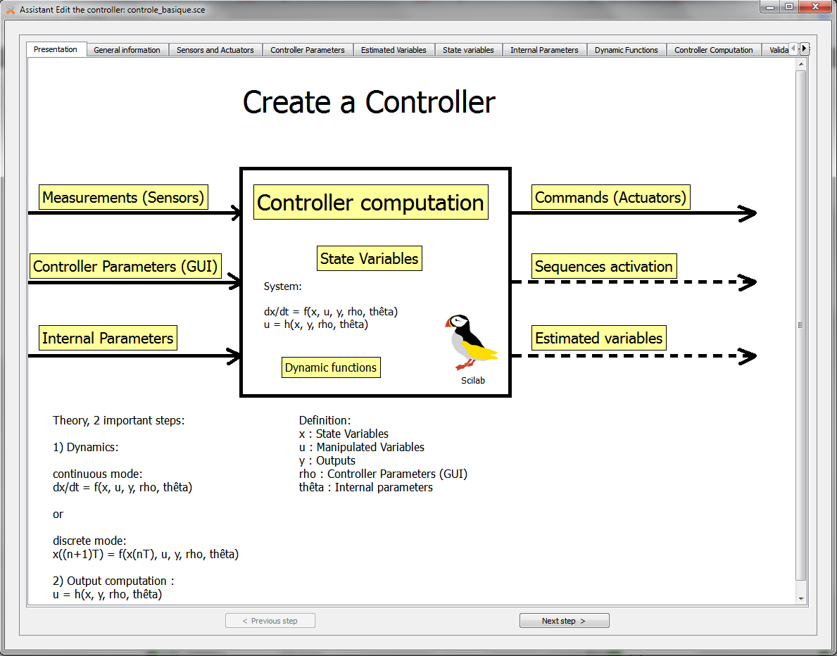
There is 8 steps to create a controller. Some are optional if you create a simple controller.
You can navigate between the different steps using the tabs or buttons Previous step and Next step.

From the main page you can go to any step by clicking on the associated yellow label.

A fied mandatory is signalized by « ** » .

Step 1 : General Information

• Name of controller (UID) ** : An controller is defined by an unique name
• Description : Descriptionof the controller.
• Continous/Discrete ** : 2 modes are availables for the resolution of Ordinary Differential Equation (O.D.E.)
• Resolution mode : Many solvers are available to approach the solution of the O.D.E with scilab.
  ode is the basic method used to approach the solution of an first order O.D.E. explicit defined by : dy/dt=f(t,y) , y(t0)=y0.
  It is an interface to various libraries, particularly ODEPACK.
  The type of problem and the method to solve it depend of the value of the first (optional) argument which could be :
  “adams” : unstiff  problems. The solver lsode of package ODEPACK is used (schema d’Adams).
  “stiff” : for stiff systems. The solver lsode of package ODEPACK is used with the schema BDF.
  “rk” : Schema of Runge-Kutta adaptatif of order 4 (RK4).
  “rkf” : Shampine and Watts formulas based on the corresponding Runge-Kutta Fehlberg of order 4 and 5 (RKF45). Good for non-stiff or mildly stiff when calculating the second member is not too costly. This method should be avoided if one is looking for a very high accuracy.
  “fix“: Identical to “rkf”, but the interface is simplified, ie only rtol and atol are communicated to the solver.
  “root“: ODE solver with root finding. The solver lsodar of package ODEPACK is used. This is an alternative of lsoda which give the possibility to look for a root of an given vectorial. See ode_root for more details.
  “discrete“: Simulation in discrete time. See ode_discrete for more détails.
• Auteur : Name of the personn who create this controller (useful if you need to contact this person for some problem or to understand the algorithm)

Step 2 : Selection of sensor and actuators

Select the sensors you will use and the actuators you want to control . When you stop ODIN, you may want to set a default value to an actuator. You must indicate this value (can be changed from the GUI).

Step 3 : Control Parameters

The control parameters are constants that can be changed from the GUI.

• Select a type Control Parameter: ** variable value, Boolean, reset (only for Tes, resets a counter).
• Give an unique name (UID) ** : There can not be two control parameters with the same name
• Unity : if an unit exist give the unit associated to this control parameter
• Value range, minimum/maximum : Area in which it is possible to vary the parameter from the GUI (to be completed only for  “Variable Value” type)
• Default value ** : value used at the start of the controller
• Description : description of the control parameter

In the GUI you can adjust this parameter in the tab “Set point” :

Step 4 : Estimated variables

Estimated variables or virtual sensors are observers . You must complete, the information here as for a real sensor.

•  Give a unique name (UID) ** : Name of the sensor, it must be unique for all sensors and actuators. ODIN does not know the difference between two sensors / actuators with the same name (registration is faulty)
• Unit : if an unit exist give the unit associated to this virtual sensor
• Value ranges, minimum/maximum : used in the experiment to see if the value is in the expected area. It will be displayed in red in the graph otherwise. Also used in the export of data to indicate whether the value is reliable or not
• Initial value ** : value used to launch the sensor, then the calculated value is used.
• Description : description of the virtual sensor
• Label : The label is only used for to export data in XML format.
• Name of the group : The group name is only used to export data in XML format

Step 5 : State variable (optional if your model is simple – ie without ODE)

This is the state variable of your O.D.E.

• Give an unique name (UID) ** : This name should be unique for each state variable
• Unit : if exists give the unit of this state variable
• Initial value ** : value used for the first loop. Then the computated value will be used.
• Description : description of this state value

Step 6 : Internal parameters

Parameters are constants that you want to identify with their properties for a better reading of the algorithm (simply call its variables k1, k2, k3 is not really clear for someone who does not know the algorithm).

• Give an unique name (UID) ** :  Each constant must have an unique name
• Unit : if exists set the unit of this constant
• Value ** : value of this parameter.
• Description : description ofthis parameter

Step 7 : Dynamic function (optional if your model is simple – without ODE and that you don’t need to define additional functions)

In this page, you can define Scilab functions you want to use later.
If you have an ODE, you must complete the lower text box that contains your system to be solved.

You can add, with lists / buttons on the left, the different es variables / parameters you defined earlier.

Strep 8 : Computation of the controller

Here you must write the computation of your actuators and of the potential virtual sensors (estimated variables). You have at your disposal all variables / parameters defined in the previous steps and the “conventional calculation functions” from Step 7.
The value of the state variables is the one after the resolution of the EDO

You can now generate your controller by going to the last tab and clicking generate. You can then display the file contents (display only, not writing) to verify that there was no problem generation (only for user knowing Scilab).

Back to the previous page