Continuous Causal States (CONCAUST home page)
Overview
Click to enlarge
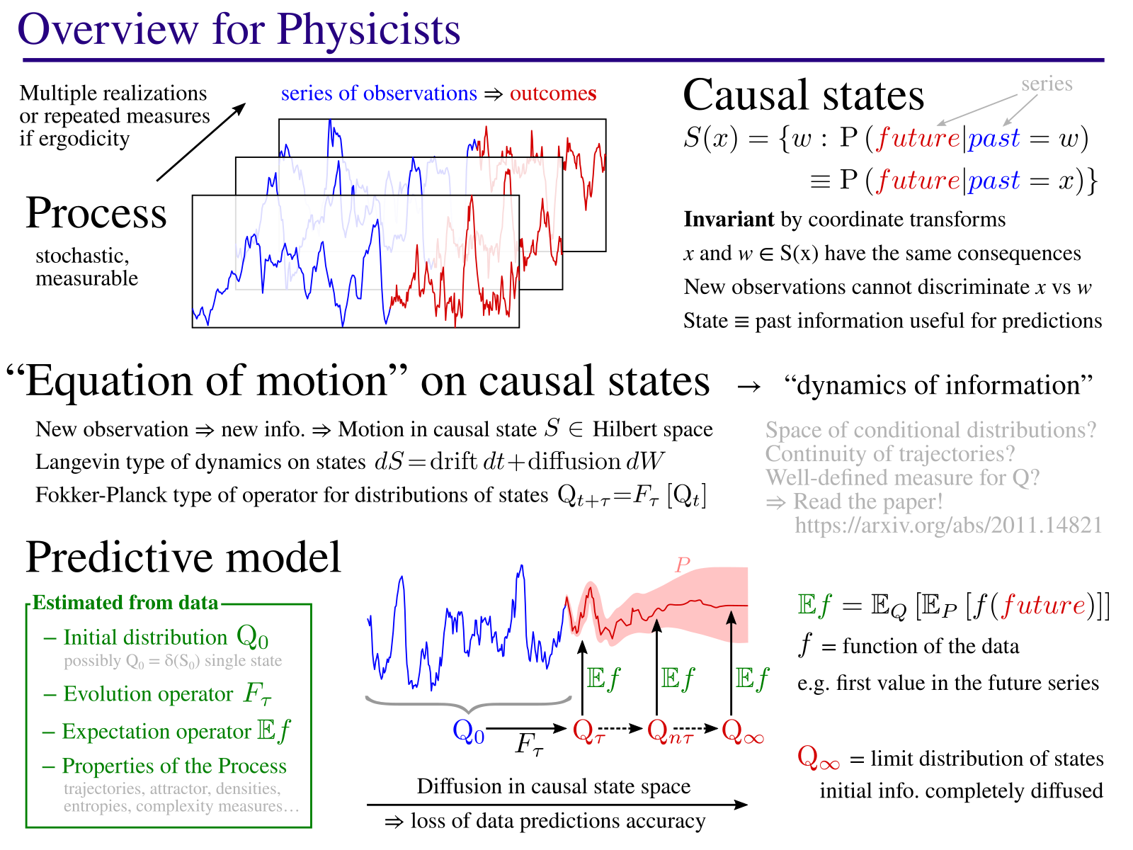
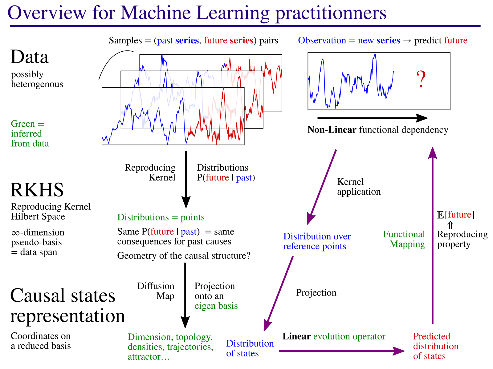
The method consists in identifying causal states: states of a process which always lead to the same kind of behaviors. The model then describes the dynamic of these states, an “equation of motion” in the causal state space. This equation describes how, starting from initial knowledge from current observations, the known information is diffused with time. As you can see in the example on this page, the method also identifies the geometric structure on which causal states evolve. This corresponds to an attractor in the case of chaotic dynamical systems. As part of this process, the method identifies the main parameters (here, 3 axes $X$, $Y$, $Z$) that best describe the evolution of the causal states.
Presentation & article
This presentation was given at the Inference for Dynamical Systems seminar series. A video replay is also available. It presents the main ideas behind the CONCAUST method.
For a full description, please refer to this article, (preprint on ArXiv).
Source code
The latest version of the source code is maintained here.
Example: solar activity
The Sun activity can be measured by counting the number of sunspots that appear each month. Periods of about 11 years are observed, which are in fact half-cycles, with a magnetic reversal between each. Prediction of these cycles is notoriously difficult. In order to test the algorithm and its ability to detect large-scale patterns, we are going to apply it to the long-term dynamic of the Sun. The algorithm is parameterized with the temporal scale of 22 years: this is how long we assume “memory” of past events can influence the present. The algorithm builds statistics on local windows of that size, in past and future. It estimates the probability distributions $P(\textrm{future}|\textrm{past})$ using reproducing kernels, then constructs a representation of these distribution as points in a reduced dimension space. Data is collected from the SILSO resource of the Royal Observatory of Belgium. The analysis script is available here.
3D representation of causal states, infered from solar cycle data. The image is dynamic and you can navigate through the structure. Click on legend items to hide / show each element.
Example: analysis
The method proposes a projection of causal states on a reduced set of most relevant parameters. Clearly, the first two, $X$ and $Y$, encode together the 11-year half-period as well as the phase along the cycle. Which is expected, given this is the main macroscopic feature of this process.
Trajectories seem to all fit on a conical structure. But what is the meaning of the $Z$ parameter, coding for the height along the cone? This parameter is identified as important by the algorithm, which puts it in third position. In fact, this parameter seems to capture the low-frequency modulation of the amplitudes known as the Gleissberg cycle. Indeed, dates on the lower or higher ends of the cone match these of the low-frequency modulation. So, the algorithm has also captured a pattern on a scale that far exceeds its immediate temporal horizon of 22 years! This demonstrate its ability to encode the dynamics of the process, not just the immediate statistical dependencies.
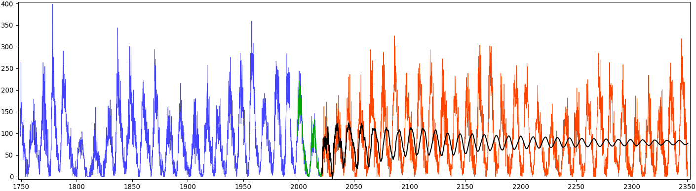
This graphic shows predictions obtained by the method on a ridiculously long time frame. The idea is to show the general behavior of the algorithm and demonstrate some concepts:
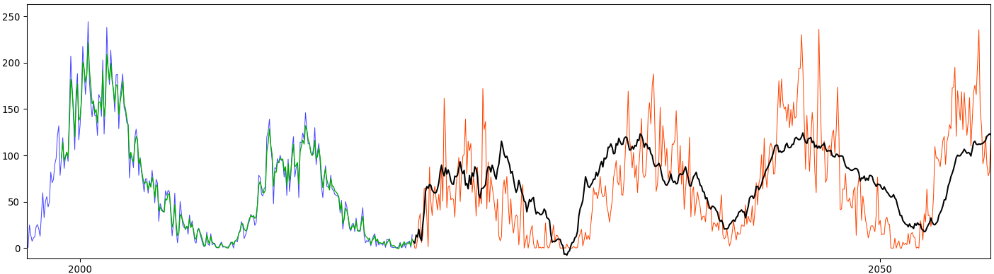
- Green values are predictions for the section of the data that corresponds to the last “future” data sequence. The last known causal state estimated from data is thus just before the beginning of the green section. As seen on the zoomed graph below, the method correctly reconstruct the training data. This yields an initial state for the predictions (black curve) from the “current” point, the very last measured data in blue. The intermediate states are also shown on the above 3D plot in green and join the blue states (estimated from data data) and the black predictions.
- A shift operator is built in order to evolve the causal states through time. As mentionned in the physics overview, for continuous-time signals the model is equivalent to an Itô diffusion in causal state space. In other words, we see the action of the operator on predictive information itself. The initial information contained in the latest observation is progressively diffused through time. Eventually, the limit distribution of the stochastic process is reached. The expectation operator maps these distributions to data, resulting in the black curve on the graphic. Eventually, all that remains is the long-term average of the data from that limit distribution.
A closer investigation of the black curve shows that progessive loss of information in action. Look at how the fine details are progressively removed from the expected values. After some time, the main feature remains, the cycles, and then these also disappear in the single average from the limit distribution. A signal processing point of view would be that of a progressively more and more restrictive low-pass filtering, until only the constant component remains. Which is, actually, what happens. Theoretically, since we are using diffusion maps parametrized to approximate the Laplace-Beltrami operator, we are projecting on eigenfunctions that form a generalized Fourier basis. In that basis, the first component (lowest frequency) corresponds to the limit distribution of the stochastic process. The shift operator takes coordinates in that basis and evolve them through time. The shift operator itself must have $1$ as eigenvalue, since it maps the limit distribution to itself, and the associated coordinates are $(1,0,0\ldots)$. The other eigenvalues have a complex module less than $1$. Repeated action exponentiate the shift operator, resulting in a well-known algorithm for extracting the main eigenvalue and vector… and in this case, converging to the limit distribution. The above 3D plot shows the second to fourth components (the constant coordinate is omitted), and the trajectories consistently reduce to $(0,0,0)$ in the center of the plot. But higher dimension components in the Fourier basis are also associated to higher frequencies. Hence, repeated exponentiation of the shift operator progressively removes these fine details and converge to the unique, constant frequency component. This is the effect we see in the data space, where the black curve shows the expected values from the trajectory in distribution space.
- In contrast, for deterministic dynamical systems represented by ODE, trajectories are unique, do not cross, so each point in phase space is its own causal state. The method then reconstructs the trajectories and the (possibly low-dimensional) attractor. In that deterministic view, the shift operator described previously would perfectly map states along the trajetories, in theory or in the limit of $N\rightarrow\infty$ observations. The expectation operator would map these trajectories in data space and the combination of both results in the Koopman operator: an operator that takes as input, an observable function $g(s)$ of the current state $s$ and which propagates it through time $[Kg](s_t)=g(s_{t+1})$. In practice the estimation of trajectories from limited data, combined with the chaotic mixing of trajectories, introduces some uncertainty on the predicted states. When this spread of predictions is added, and if we assume continuous trajectories, we recover an inhomogenous Itô diffusion model on the form $s_{t+dt} = a(s_t)dt + b(s_t)dW$ and a related stochastic evolution operator. In either case, we may want to produce valid trajectories sampling the attractor and these do not converge to the expectation of the limit distribution. That average needs not be a valid state and may lie outside the attractor, as is the case in the above 3D plot.
Both theoretical developments and practical engineering are needed to properly estimate $a(s)$ and $b(s)$, which the current code is not yet able to do. Then, proper trajectories could be produced and their ensemble average should match the black curve. In the mean time, a surrogate trajectory in causal state space is shown as the orange curve in the 3D plot. This empirical attempt to maintain a valid trajectory is based on nearest-neighbors quasi-convexity constraints, with a slight tolerance on the convexity. Each application of the shift operator is then projected to the nearest point of that nearly-convex region, so the resulting trajectory remains on the attractor. The expectation operator is applied as usual, resulting in a trajectory in data space that does not display as many extreme events. Still, this imperfect method allows to visualize potential trajectories produced by the algorithm, which can be quite informative. In this example, we see that the Gleissberg cycle seems to be properly reproduced. The comparison with the expected (black) values is also interesting. While the black average progressively loose details, this is not the case for the orange trajectory. This corresponds to the orange curve remaining along the attractor in the 3D plot, while the black curve deviates towards the center of the cone (this is easier visualized by clicking on the legend to hide the measured data). Eventually, when the black curve converges towards its limit value, the trajectory on the attractor has become completely uncorrelated with its initial condition. Of course, at that point (and much before), the orange curve details have also become completely irrelevant.
Connexions
The action of the shift operator was analyzed above in conjunction to Fourier analysis. In the deterministic dynamical system interpretation, more connexions can be made, especially with Taken’s time-lag embedding technique. Assuming $d$ represents a data time series. A vector of time-lagged values is constructed $X_t = (\ldots, d_{t-n\tau}, d_t)$ with $n\lt N$ the number of components to retain. There is abundant litterature for how to best select the embedding dimension $N$ and the lag $\tau$ based on data. The dynamic of the process is then studied by looking how $X_{t+1}$ relates to $X_t$.
In contrast, the Concaust method takes the full data series, without subsampling, $x_t = (d_{N\tau+1}, \ldots, d_t)$ and similarly for the future $y_t = (d_{t+1}, \ldots, d_{t+M\tau})$. If no causal decay is selected (see the paper) and if a lag of $\tau=1$ is choosen, then we get the same $X$. In order to study the evolution of $X_{t+1}$ with respect to $X_t$, the Kernel Koopman operator is a related method that represents the conditional distributions $p(X_{t+1}|X=x_t)$ using reproducing kernels. In contrast, we represent the distributions $s_t \equiv p(Y_t|X=x_t)$, with full future series to discriminate the influence of the past series. We then explicitly construct $P$, the shift operator $s_{t+1} = [Ps](t)$, in that distribution space. In addition, we are not decomposing the data on Koopman modes. Instead, we are decomposing the data on a variant of the Diffusion Map algorithm, adapted to this context. As we have seen above, the states are then expressed on a generalized Fourier basis. Thus, instead of choosing a particular period $\tau$ for probing the signal, as in time-lag embeddings, in our case all frequencies are evolved simultaneously and acted upon by the shift operator. Another advantage of using diffusion maps is that, with the choosen parametrization, the method cleanly reconstructs the geometry of the attractor without influence from the sampling density.
In addition, the composition of kernels allows us to seemlessly merge heterogenous data sources, and to choose different time scales for each data source. Compared to time-lag embedding, this would be like choosing different $\tau$ and $N$ parameters for different time series, while still building a unique $X$ in a consistent way, even for mismatched data types.
Open questions
One recurring issue with current machine learning and data analysis methods, is that of their interpretability. The above connexions hopefully point towards a good degree of interpetability for the Concaust method. Yet, some additionnal theoretical developments are necessary and, perhaps more importantly at this stage, more applications to concrete processes. For processes that can be described by a dynamical system, then Concaust should be able to recover relevant variables for their dynamic. By analogy with phase spaces of dynamical systems, these variables would not correspond to the causal states themselves, but rather to the dimensions found for describing the causal states.
Concaust is a kernel-based method, limited in applicability both by the size of the data sets and by the kernels themselves. For now, the code uses the Gaussian kernel for convenience, but this may not be adequate for some situations. Any kernel could be used, including that for strings of text, for graphs… and heterogenous data can be composed. What are the limits of this approach? What are the characteristics of data sets, which make them suitable for analysis by Concaust?
Nothing is assumed as to why information is progressively lost for making predictions. Ideally, we’d like to quantify the properties inherent to the physical process being investigated. But another source of dissipation comes from the RKHS representation itself: when the true future state lies outside the data span, it is not representable by the shift operator. Currently, the code has no built-in method to discriminate these effects. But when the process dynamic can be expressed by a few descriptive variables and a low-dimension attractor is found, we can hope that all useful information is also contained in these variables and low dimension. Then, a possible way to separate the loss due to the representation part from the inherent mixing due to the chaotic dynamic, would be to investigate the dependency with the data set size.
How to detect anomalies? These should stand out as states of low probability… but so are outliers. Yet, the method has promising analysis capabilities for this. For example, hide the predicted trajectories and keep only the measured data and dates in the above 3D plot. See that path between 1778 and 1788, right through the middle of the plot? Was that data badly measured, or is the attractor more complicated with occasionnal rare paths? Anomalies are also found and clearly stand out in the El Niño data. In that case, these anomalies correspond to extreme events.
This list could continue endlessly with connexions to machine learning, with multi-scale analysis, with extension to spatio-temporal systems… Of all these possible research directions, there is a huge theoretical development to be made on the thermodynamics of information. See the section on general objectives. Causal states group system configurations by predictive information equivalence, rather than by energy classes. Their evolution obeys laws that can be seen as transformations of information, instead of transformation of energy. The above connexions show we can study the convergence to a limit distribution of causal states by a diffusive process, which parallels the convergence to a thermodynamic equilibrium distribution that would also be reached by a diffusive process. Work is ongoing in the team to extend and formalize these analogies and we welcome new collaborations
Want to join us?
Do not hesitate to contact us if you had the patience to read through this long text, especially if you are highly motivated rather than bored at this point! We can:
- Provide post-docs and other temporary positions. Some may be announced in the job offers section of this site, but we could sometimes create new positions. We can support your application for a grant to funding agencies and in particular the European Union (e.g., Marie-Curie fellowships and ERC starting grants).
- Support you for a permanent position at Inria. This is a serious opportunity. We are currently in the process of creating a team around these issues, so recruiting colleagues to complement that team is our priority.
- Collaborate in any case. With the current sanitary situation international travels are not easy, but we’d be pleased to discuss online in the mean time.